4.1. How to Download the data with Copernicus Browser

4.1.1. Why Sentinel-2

The Sentinel-2 mission is part of the Copernicus program through which two satellites were launched with the aim of providing high resolution multi-spectral images of the Earth’s surface. The two satellites are placed 180° from one to the other on a polar sun-synchronous orbit at around 800 km from the earth offering a revisit time of the same area at the equator of 10 days. In this way the constellation composed by the two satellites permits a revisit time of 5 days, a low revisit time is fundamental when trying to monitor phenomena that changes through time like a flooding event or a wildfire. Images captured by Sentinel-2 are composed of 13 spectral bands, some of which are in the visible range while others are infrared. With this composition it is possible to analyze things like land cover, water quantity and quality, vegetation health, soil composition etc. The spatial resolution of Sentinel 2 varies between 10 to 60 m depending on which band we are referring to, in this way it is possible to retrieve detailed observations Talking about coverage, Sentinel-2 satellites offers a swath width of 290 km; this means the width of the area on earth that these satellites can capture passing a single time over an area very noticeable allowing to reduce data mosaicking. Another important feature of data acquired via Sentinel-2is that are accessible for free and available to the public.

4.1.2. Search for Sentinel-2 images in Copernicus Browser

In order to proceed in this lecture it’s necessary to possess the EMS vector data: “EMSR468_AOI05_DEL_PRODUCT_areaOFInterestA_r1_v1.json” downloaded in lecture 3 . Before browsing the image archives, log in to your account in Copernicus Browser (Fig. 4.1.2.1) . Click on Login (1) then fill in the Email (2) and Password (3) fields with the credentials you used to register in Chapter 2.1.2.1 of lecture 2. As the last step, click on LOGIN (4), if everything is correct your name will appear on the top right corner of the sidebar.

Fig. 4.1.2.1 – Log in to Copernicus Browser

Once logged in; we are going to take advantage of Copernicus Browser flexibility to find the data we are interested in and to upload the area of interest (AOI). To do so, set the following parameters in the SEARCH tab (Fig. 4.1.2.2): check the L2A box (1); set cloud coverage to 40% (2); set the TIME RANGE to 28-09-2020 to 04-10-2020 (dd-mm-yyyy), in this case there is no need to modify the hours and minutes range (3). This procedure will narrow down the data that will be shown to us. Given the size of the Copernicus Browser entire dataset it would have been impossible to find the data we are interested in without this procedure. Then, set the area you are interested in by clicking on (4) and choose the “Upload” method (5). This will allow downloading data relative to a limited area reducing the space needed to store them. At this point click on the area surrounded by the gray dotted line (6) and look through your files searching for: “EMSR468_AOI05_DEL_PRODUCT_areaOFInterestA_r1_v1.json” (7) (this file was downloaded in lecture 2 . A .json file (JavaScript Object Notation) is a flexible and lightweight format used to store various information that can be easily converted into JavaScript objects. As soon as the area has been uploaded click on Open (8). Alternatively, you can just drag and drop the file in the designated area (6).

Note

You can read more about JavaScript Object Notation here .

Fig. 4.1.2.2 – Set AOI and search parameters

Once you have done it, the highlighted blue polygon representing the area of interest will be shown like in Fig. 4.1.2.3 . Now click on Search (1).

Fig. 4.1.2.3 – Area of Interest

4.1.3. View and display Sentinel-2 images in Copernicus Browser

You will now see the image tiles covering the AOI (Fig. 4.1.3.1) . We need to look for a product that totally covers the uploaded AOI. The characteristics of the desired product are illustrated in (Fig. 4.1.3.2) . You can select it either by clicking directly on Visualize from the sidebar (1) or by selecting the image tile that better covers the AOI (2) and then, clicking on Visualize (3) inside the spawning window. .. note:: If the area we are interested in is not completely covered by a single tile it is also possible to download more than a tile and combine them through a procedure called data mosaicking.

Fig. 4.1.3.1 – Tile visualization for Satellite image(s)

Fig. 4.1.3.2 – Desired image details of post flood event in Vercelli

Now change the default visualization from True color to NDWI (1) (Fig. 4.1.3.3) ; then click on Add to (2) and finally click on Add to Pins (3). If everything was done correctly you will see a notification over the icon (4) indicating that you have pinned one product. Click on the pin icon (4).

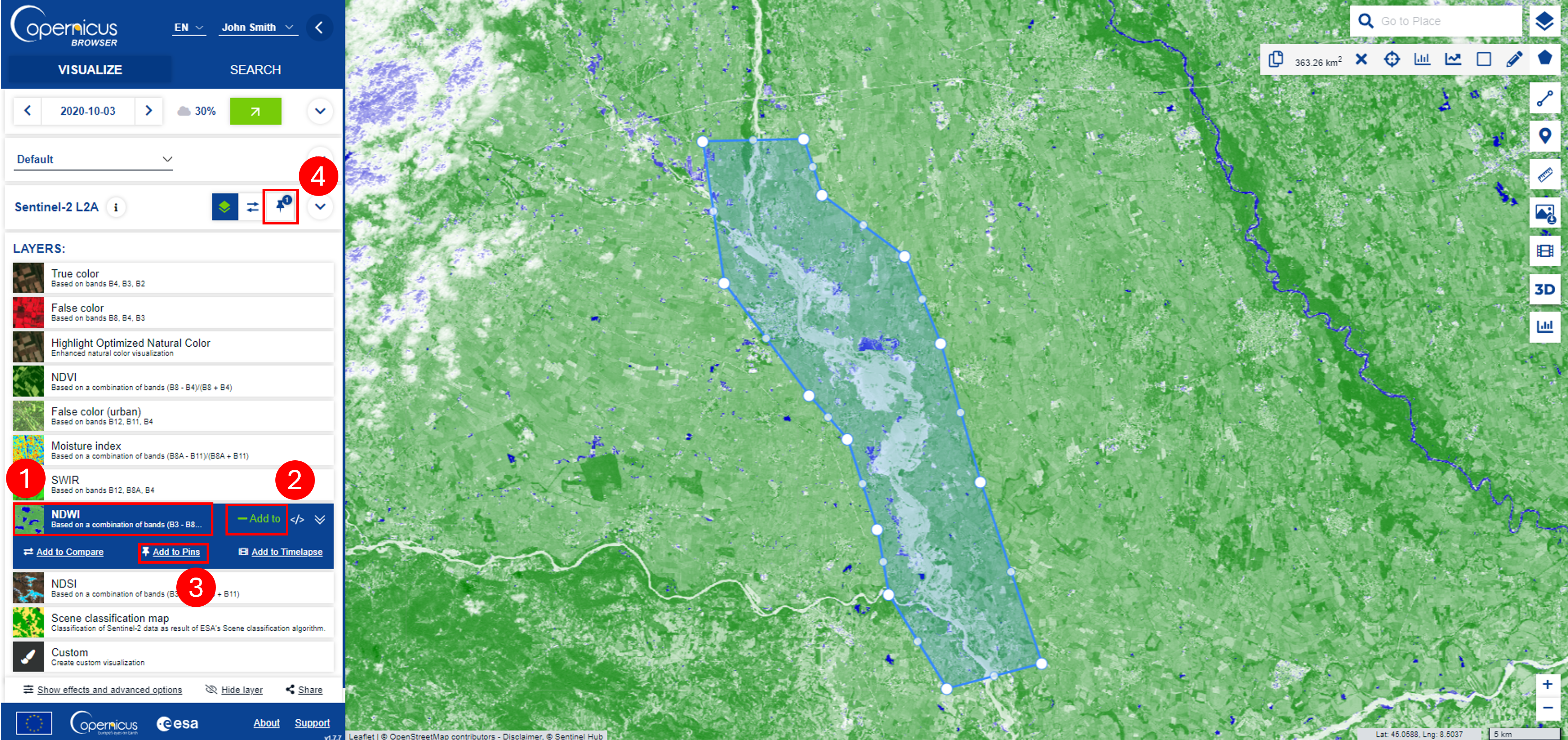
Fig. 4.1.3.3 – Post event Satellite image visualization in Copernicus Browser

4.1.4. Images Comparison in Copernicus Browser

The following procedure will allow a comparison between two or more products. This operation can be useful to understand if the considered products are the one that better suits our requirements. The comparison already started when you clicked on pins. As shown in Fig. 4.1.4.1 , by clicking on (1) you can edit the image name (preferable to leave it as default). Instead, clicking on icon (2) and then on icon (3) will allow you to add a description to your product. Now set in (4) the date prior to the event (corresponding to 28-09-2020).

Fig. 4.1.4.1 – Pinning Sentinel-2 Post event image (28-09-2020)

Ensure that you are visualizing the NDWI and add this new product to the pins panel as we have seen in the step before and open the pins panel (1). (Fig. 4.1.4.2)

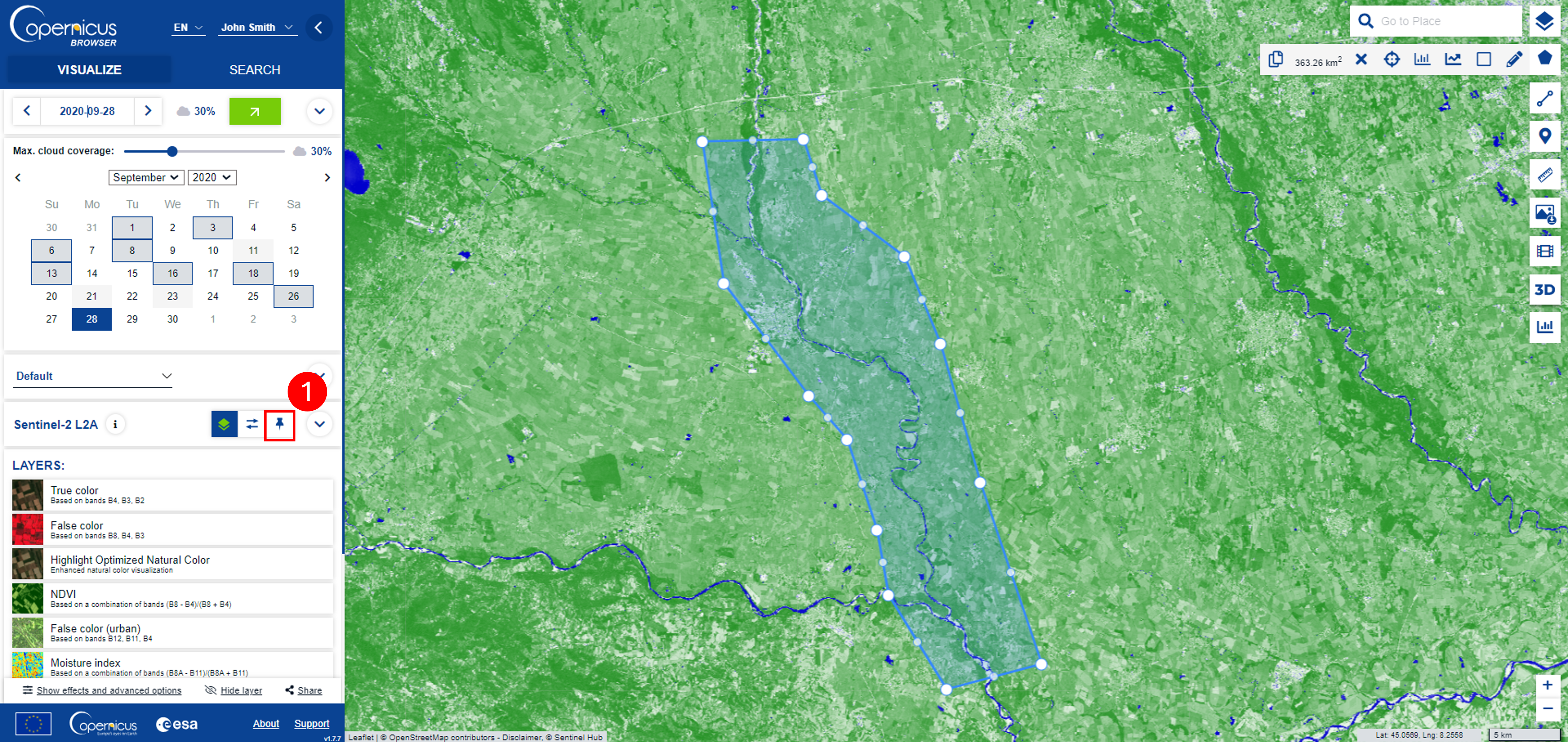
Fig. 4.1.4.2 – Pre event Satellite image visualization in Copernicus Browser

Clicking on the icon (1) for both images (Fig. 4.1.4.3) , enables the Satellite images to be compared through the compare panel that you can open by clicking on the icon with the two arrows (2).

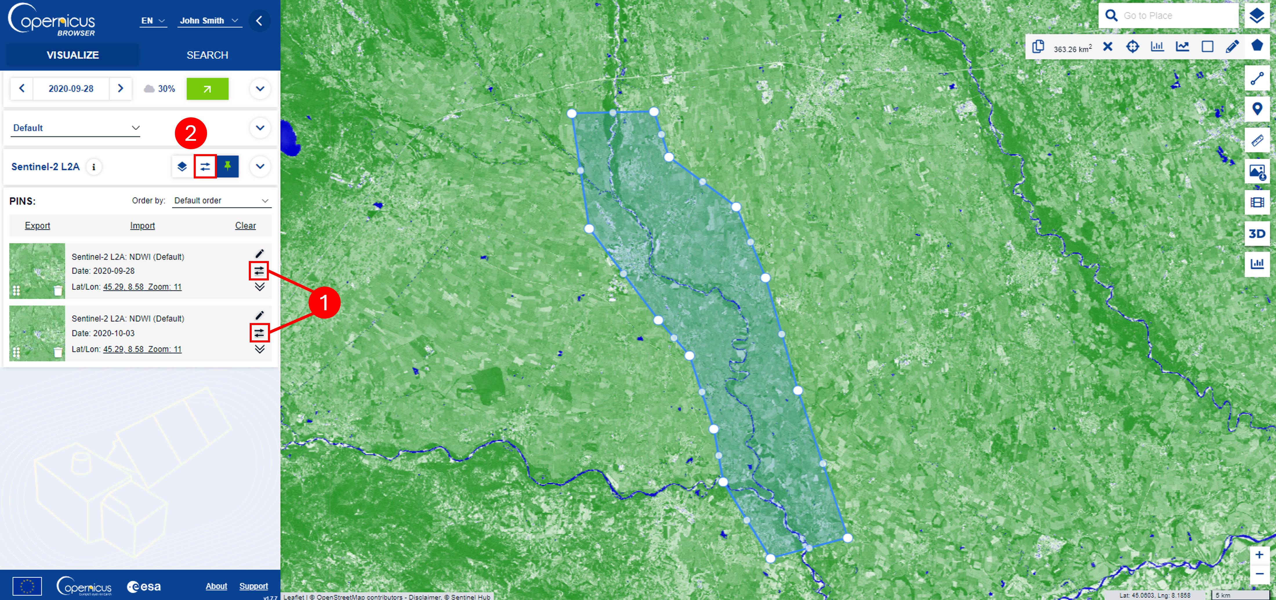
Fig. 4.1.4.3 – Pinning Pre and post event images

As shown in Fig. 4.1.4.4 set the Effect (1) from the default value of Split to Opacity, now, by using the interactive bar (2) you can decrease and increase the transparency.

Note

Using the Split option for the comparative visualization will allow you, through the use of the same interactive bar, to hide and illustrate the bottom layer (like you are flipping and turning a book page from right to left).

Fig. 4.1.4.4 – Vercelli’s NDWI Comparison in Copernicus Browser

4.1.5. Evolution of flooded area “Timelapse” in Copernicus Browser

What kind of image properties do you think have the major role with respect to the term “flood evolution”? Since the term evolution is related to time, the best answer is Temporal. We can follow the comparison in Copernicus Browser in the last section , but it is insufficient in case we have tens of images. Copernicus Browser provides the solution for such a case (Fig. 4.1.5.1), through what is called Timelapse; to use this functionality, first you must go in the Layers Panel by clicking the icon (1) then you need to click on the Create time-lapse animation symbol (2).

Fig. 4.1.5.1 – Activate Timelapse in Copernicus Browser

Warning

The time-lapse will illustrate the last visualization that has been used. Be sure you are visualizing the NDWI before proceeding.

A new window in which you can view and download the time-lapse animation will spawn. Here (Fig. 4.1.5.2) a couple of parameters must be set:

• Time range: the period that you want to detect the evolution of the flooded area. In our case we want to set it as: 2020-09-28 - 2020-10-03 (1).
• Min. tile coverage: how much is the coverage percentage of the tile with respect to the area of interest. Set to 100% (2).
• Max. cloud coverage: exclude images with cloud coverage lower than the value you have set. Set it to 100% (3) to have as many images as possible, we will remove some manually later.
• Select 1 image per: here we choose the interval between images, we will leave the default configuration which is: day (4).

Now you might want to deselect some images. Here, for example, we will exclude the first one since its cloud coverage is too high and it is almost impossible to distinguish our area; to do so, click on (5) to un-check the corresponding product. To visualize the time-lapse animation online, with the integrated visualization click on (6). In order to download the animation, click on Download (7). Once you have done, click on (8) to close this window.

Fig. 4.1.5.2 – View and download Timelapse

4.1.6. Download Sentinel-2 images

Now that you have closed the time-lapse click on (1), to download the image as shown in Fig. 4.1.6.1 . Choose the analytical panel (2) to set the image format to TIFF (3) (Tagged Image File Format). The .tiff format is a popular file format used to store raster data, it allows lossless compression (there is no loss in image quality while compressing the file) and storing images with different color depths.

Note

more information about .tiff format can be found at this page .

Set the image resolution to HIGH (4) and the coordinate system to WGS84 (5). At this point you can choose the layers (6) and bands (for this lecture select all of them) (7) that you like to save, remember that by toggling Clip extra bands (8) only the first 3 bands will be included in the image. Once you are done, you can download your images through the Download button (9).

Fig. 4.1.6.1 – Download Sentinel-2 images from Copernicus Browser