2.1. Access to Copernicus Satellite images for free
2.1.1. Remote Sensing and Earth Observation
Remote Sensing is the science that studies how to acquire information about an object without being in contact with it. Usually the object of remote sensing is the Earth itself, in this case we talk about Earth Observation.
2.1.1.1. Satellites
In order to acquire our observations we use sensors mounted on satellites. Satellites are objects placed into orbit around a celestial body. There are different orbits varying in shape, size, and orientation depending on factors such as altitude, inclination, and eccentricity, we will report here some of them:
- Geostationary orbit (GEO): satellites placed in this kind of orbit are situated approximately at an altitude of 35,000 km and appear stationary relative to a fixed point on the Earth’s surface providing continuous coverage of the region around that point
- Low Earth orbit (LEO): satellites placed in this kind of orbit range from 160 km to 2000 km above the Earth’s surface, these low altitudes allow high resolution and rapid revisiting of the same region
- Medium Earth orbit (MEO): satellites placed in this kind of orbit are placed in a distance ranging between the one of the low Earth orbit and the one of the geostationary orbit. Satellites here offers a trade off between revisit time and coverage
- Polar orbit: satellites placed in this kind of orbit pass over the Earth’s poles
- Sun-synchronous orbit (SSO): satellites placed in this kind of orbit precess at a rate that matches the Earth’s orbital motion around the Sun, meaning that with every orbit, the satellite passes at the same solar time over any given point on the Earth’s surface. Sun-synchronous orbit represents a specific case of polar orbits.
Through satellites we can achieve a global coverage and a consistent temporal sampling, often requiring little to no cost for the final users as it happens for the European Copernicus Project.
2.1.1.2. Image Acquisition
What we measure is the electromagnetic energy that the Earth emits or reflects. Electromagnetic energy is a combination of an electrical and a magnetic field, the former varying in magnitude perpendicularly to the travel direction, while the latter being oriented in such a way that it completes the right-handed triad. What characterizes the electromagnetic energy is its frequency (f) and wavelength (\(λ\)), the two are connected by the relation:
where v is the speed of the wave. In the vacuum the speed of both electrical and magnetic fields is equal to the speed of light (c). Given these notions, the idea is that we can measure the ratio between reflected and emitted energy as a function of wavelength and retrieve the unique pattern corresponding to each material that takes the name of spectral signature. After that, by comparing an observed signature to a known one we will be able to recognize which material it corresponds to.
2.1.1.3. Image Characteristics
Processing levels Products can be classified based on the level of processing they undergo, in particular we talk about 5 levels:
- Level 0: also referred as raw data, these data are only corrected from the transmission errors and are usually not suitable for analysis without further processing.
- Level 1: includes sensor distortions corrections, geometric corrections, and radiometric corrections. This is the kind of product we are going to work with in these lectures.
- Level 2: In this stage, algorithms to enhance some characteristics of the data are applied. Examples of resulting products can be surface elevation maps or vegetation indices.
- Level 3: Products in this level, also referred as Gridded Data Products, are composed of thematic products such as average temperature maps or urbanization growth rate maps. These products are derived from level 2 products which are aggregated, averaged or interpolated.
- Level 4: In this last stage, data are integrated with other products and modeled to give prediction/forecasting. Some examples can be seen in the use of urbanization growth forecasting used to predict the energy production that will be needed to sustain a certain area.
Spatial Resolution The spatial resolution refers to the size of the smallest feature that can be represented and specifies the pixel size of satellite images at the Earth’s surface. Depending on their image pixel size, remote sensing cameras are classified as:
- Very high spatial resolution: < 1 m
- High spatial resolution: 1 - 5 m
- Medium spatial resolution: 5 - 100 m
- Low spatial resolution: > 100 m
In this lecture we will use multispectral medium resolution imagery for land services provided by Sentinel-2 satellites (twin satellites Sentinel-2A and Sentinel-2B). Those images will allow us to distinguish houses but certainly not people.
Temporal Resolution Temporal resolution is defined as the minimum span of time between two consecutive observations on the same site. It is very important for monitoring. For a satellite it is the length of time it takes it to complete an orbit cycle. In order to monitor phenomena like a volcano eruption a temporal resolution of 1 day may be enough while in traffic monitoring an hourly or even less temporal resolution may be needed. Sentinel-2 constellation will provide, with one satellite, a temporal resolution of 10 days at the equator.
Spectral Resolution Spectral resolution is defined as the number of spectral bands (Fig. 2.1.1.1) in which we divide our spectral range. With Sentinel-2 satellites we can capture imagery in 13 spectral bands depending on the spatial resolution.
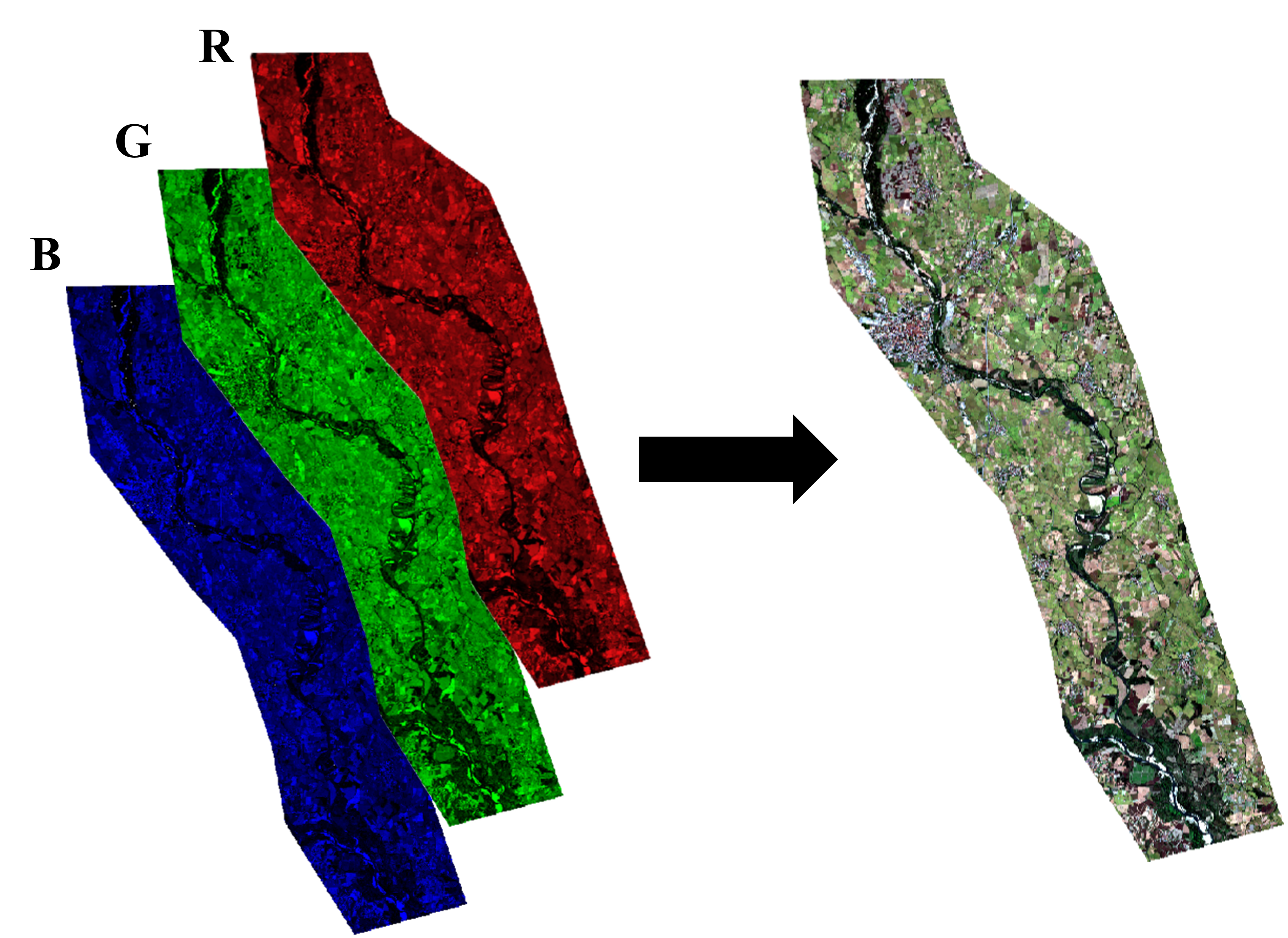
Fig. 2.1.1.1 – Example of multiband image
2.1.1.4. Image Analysis
Image indices are images derived from multiband images. The resulting product highlights a specific phenomenon in the area of interest and allows a better comprehension of the phenomena. Some of the indices that can be seen in Copernicus Browser are shown in Fig. 2.1.1.2:
- NDVI: Normalized Difference Vegetation Index (1) it is a widely known index used to quantify green vegetation. It normalizes green leaf scattering in Near Infra-red (NIR) wavelengths with chlorophyll absorption in red wavelengths. It can be computed as: NDVI = (NIR - RED) / (NIR + RED)
- NDMI: Normalized Difference Moisture Index (2) can be computed as: NDMI = (NIR-SWIR) / (NIR+SWIR) where SWIR stands for shortwave infrared and it is used to detect changes in the water content of the leaves. The amount of water inside a leaf is in fact responsible for the reflectance in the SWIR interval.
- NDWI: Normalized Difference Water Index (3) can be computed as: NDWI = (GREEN - NIR) / (GREEN + NIR). Water bodies have in fact shown a sensible light absorption towards the part of the electromagnetic spectrum between visible and infrared. This index may overestimate water bodies since urbanized areas can also reflect in those bands.
- NDSI: Normalised Difference Snow Index (4) can be computed as: NDSI = (GREEN - SWIR) / (GREEN + SWIR) where SWIR stands for shortwave infrared. This index can also be used as a tool to distinguish between snow cover and clouds since both absorb light in the SWIR but generally only clouds reflect the visible light.
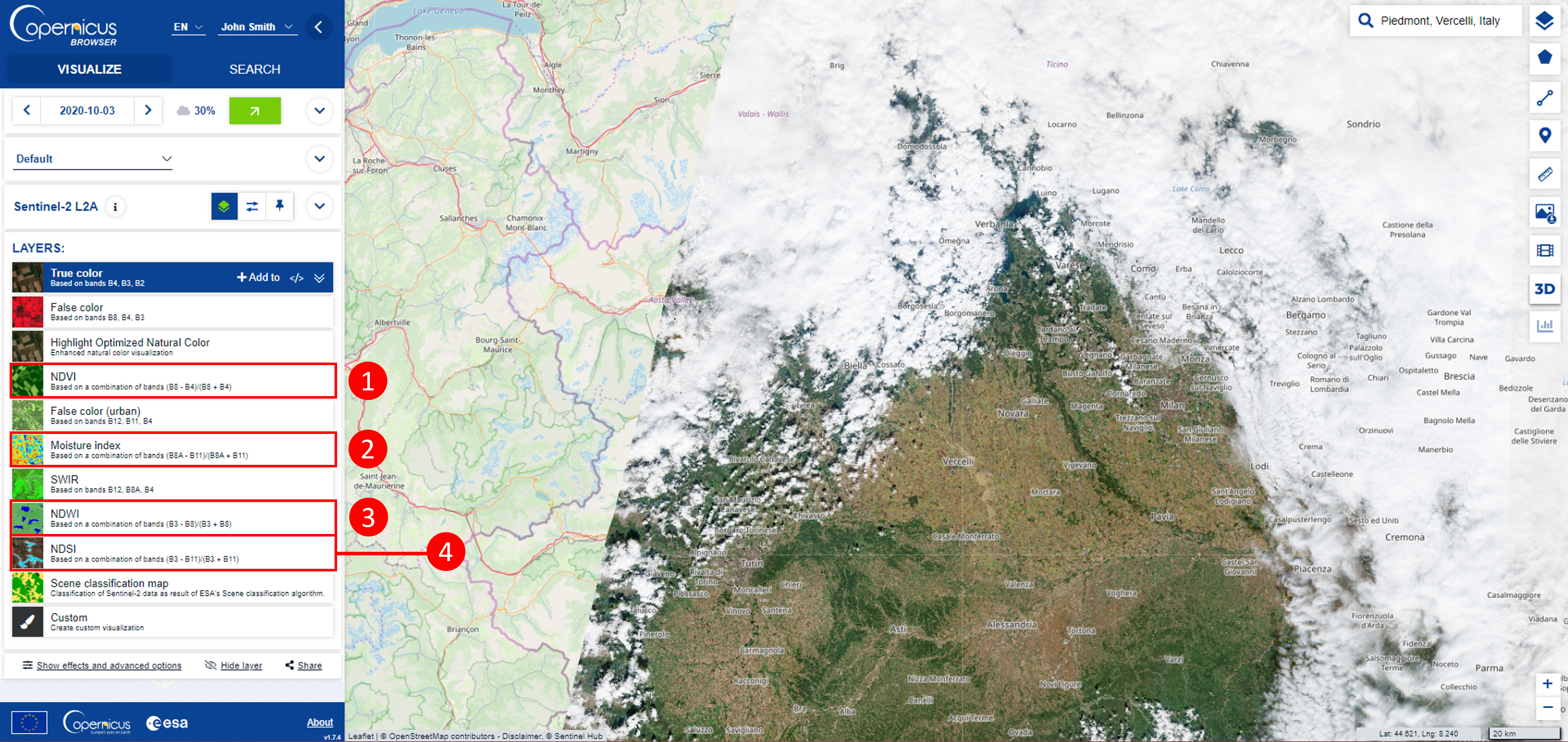
Fig. 2.1.1.2 – Copernicus Browser Indices
2.1.2. Copernicus Browser
Copernicus Browser combines a complete archive of Sentinel-1, Sentinel-2, Sentinel-3, Sentinel-5P, ESA’s archive of Landsat 5, 7 and 8, global coverage of Landsat 8, Envisat Meris, MODIS, Proba-V and GIBS products in one place and makes it possible to browse and compare full resolution images from those sources. Copernicus Browser interface (Fig. 2.1.2.1) is composed of three main sections, on the left there is the sidebar (1), in the center there is the map (2) and on the right of the screen there is the tool bar. The sidebar functionality will be explained further down the lecture. In the map section it is possible to visualize selected products and to move around and zoom in and out checking the results of a selection. Lastly, in the toolbar it is possible to zoom to a specific location (3) and to make use of many tools. For clarity purposes the tools icons have also been reported on top of Fig. 2.1.2.1 :
- Layers (4)
- Create an area of interest (5)
- Draw a line (6)
- Make point of interest (7)
- Measure (8)
- Download image (9)
- Create timelapse animation (10)
- Visualize terrain in 3D (11)
- Histogram (12)
Note
In case you want to read the documentation it can be reached through the following link Copernicus Browser Documentation .

Fig. 2.1.2.1 – Copernicus Browser Interface
An example of use of the Layers tool is shown in Fig. 2.1.2.2. By clicking on the corresponding icon (1) it is possible to choose different base maps and layers showing different aspects such as roads, borders of countries and regions, water bodies etc. In the left image only the Sentinel-2 Mosaic layer has been activated (2) while in the right one the OSM Background, water bodies, roads and labels layer have been activated (3) but both images show the same area.
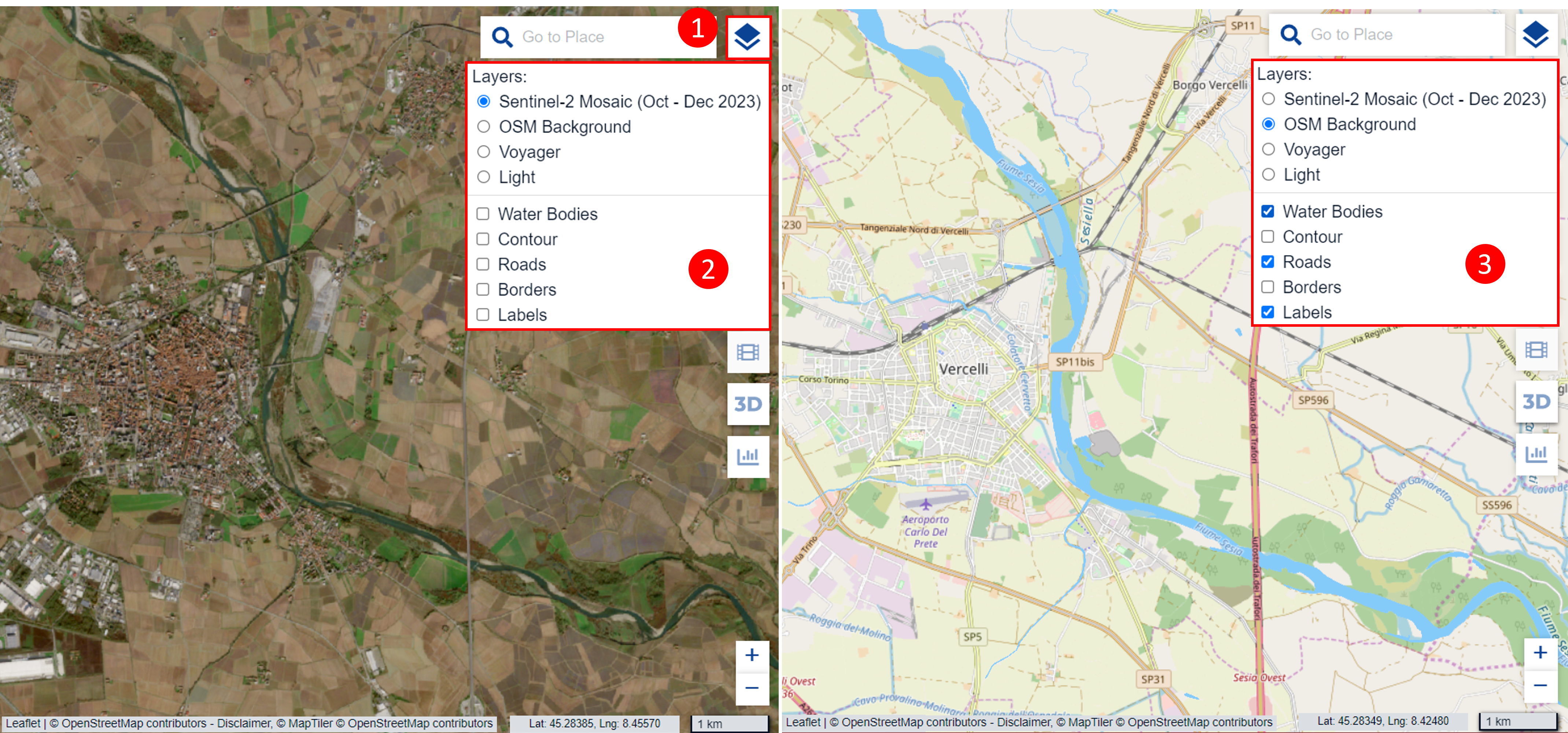
Fig. 2.1.2.2 – Layers Tool
An example of use of the Create an area of interest tool is shown in Fig. 2.1.2.3. By clicking on the corresponding icon (1) it is possible to choose different ways of drawing the area, in the top part of the image a rectangular area is shown. In order to draw it, click on the squared icon (2) then click on a point in the map, this action will fix the first vertex of the rectangle, by clicking on another point the rectangle will be drawn (3). You will be able to visualize the contained area and copy it (4). Clicking on the x icon will delete the area selection (5) while clicking on the crosshair icon will center the map on the selected area (6). In the bottom part of the image a second way of drawing the area is shown, by clicking on the pencil icon (7) you can draw a polygonal area (8), all other functionality remains the same.
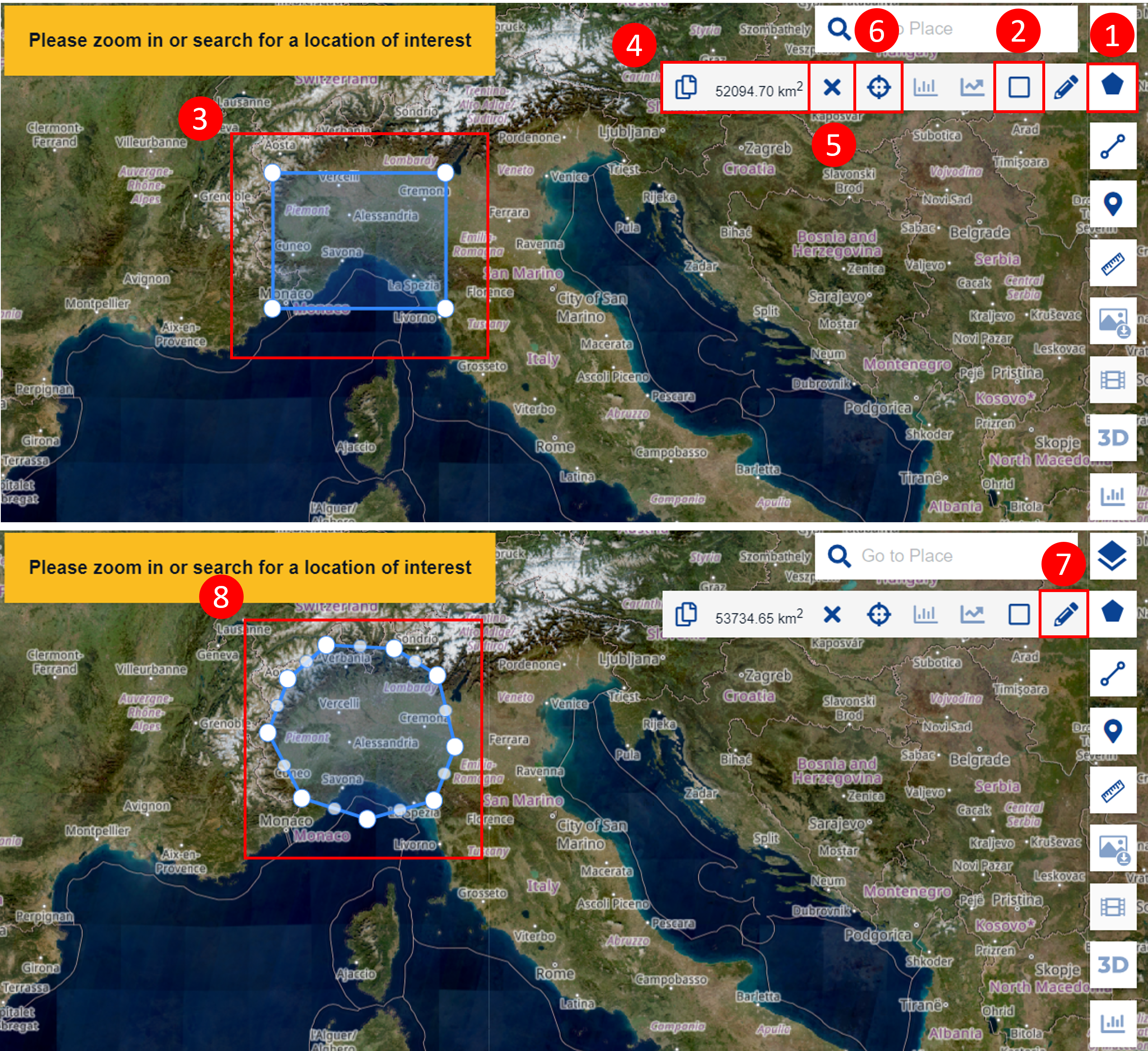
Fig. 2.1.2.3 – Draw Area pt.1
In order to utilize the last two tools shown in Fig. 2.1.2.4, it is needed to select a product (in later chapters it will be shown how to do so). By clicking on Spectral explorer (1) a new menu will open up from which it is possible to check the spectral signature of the selected area (averaged over all the pixels within the area itself) (2). It is also possible to add to the graph other known signatures that can be activated by clicking on the legend entries at the bottom of the graph (3) in order to make comparisons. By clicking on Values (4), the band’s values will be visualized in a table format (5). The last tool is not available for true color maps and some indexes, in this case we use it over the NDWI index which is supported (how to select a specific index will also be shown in later chapters). By Clicking on the Statistical info/feature info Service chart tool (6), a new menu will open up from which it is possible to check the index change over time in the selected area (7). Once an area has been selected it is possible to click on the Histogram tool (8) to have an insight of the data distribution (9).
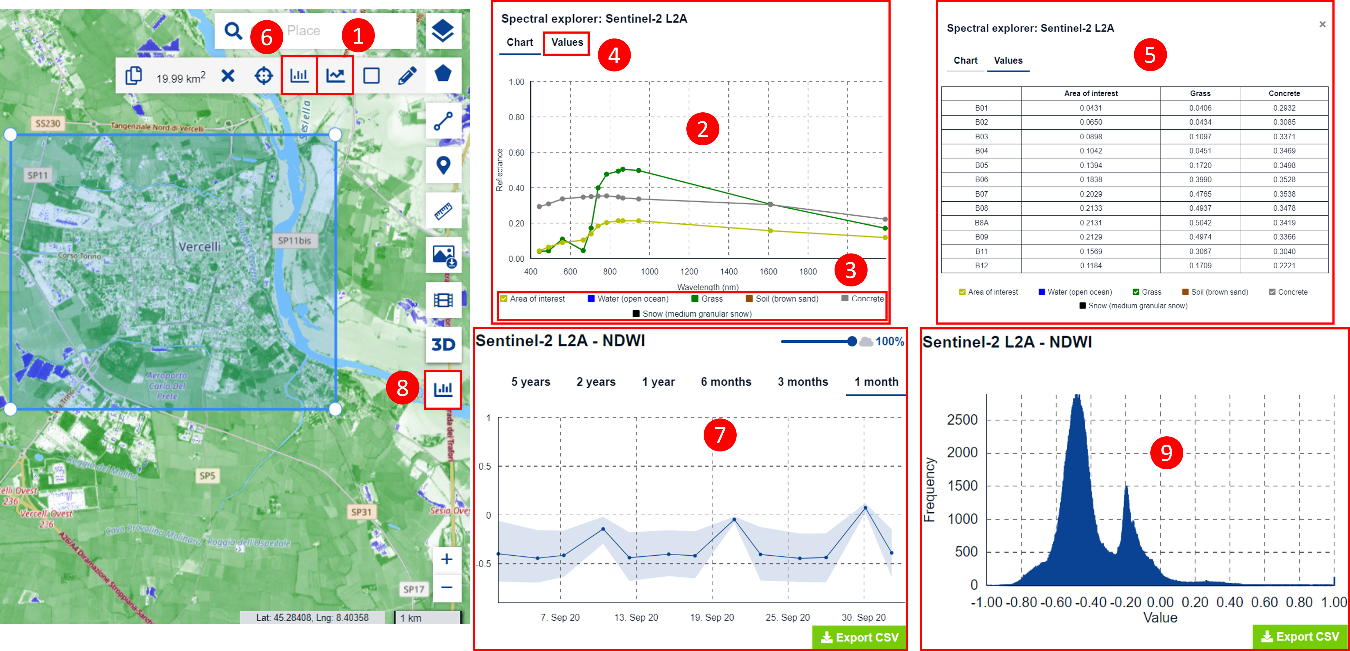
Fig. 2.1.2.4 – Draw Area pt.2
By clicking on the Draw a line tool (1) (Fig. 2.1.2.5) you can click on the maps and draw lines, of those lines you can check the length but most importantly you can click on Elevation profile (2) to open a graph representing the elevation with respect to the distance (3). Another tool is the Mark point of interest, by clicking on it (4) you can then click on the map and place a marker, you can check the index change over time in the selected point by clicking on the Statistical info/feature info Service chart in the same way as with the Create an area of interest tool. With the Measure tool (5) it is instead possible of measuring length and areas over the maps. .. note:: Download image, Create timelapse animation and Visualize terrain in 3D tools will be shown respectively in lecture/chapter xxx
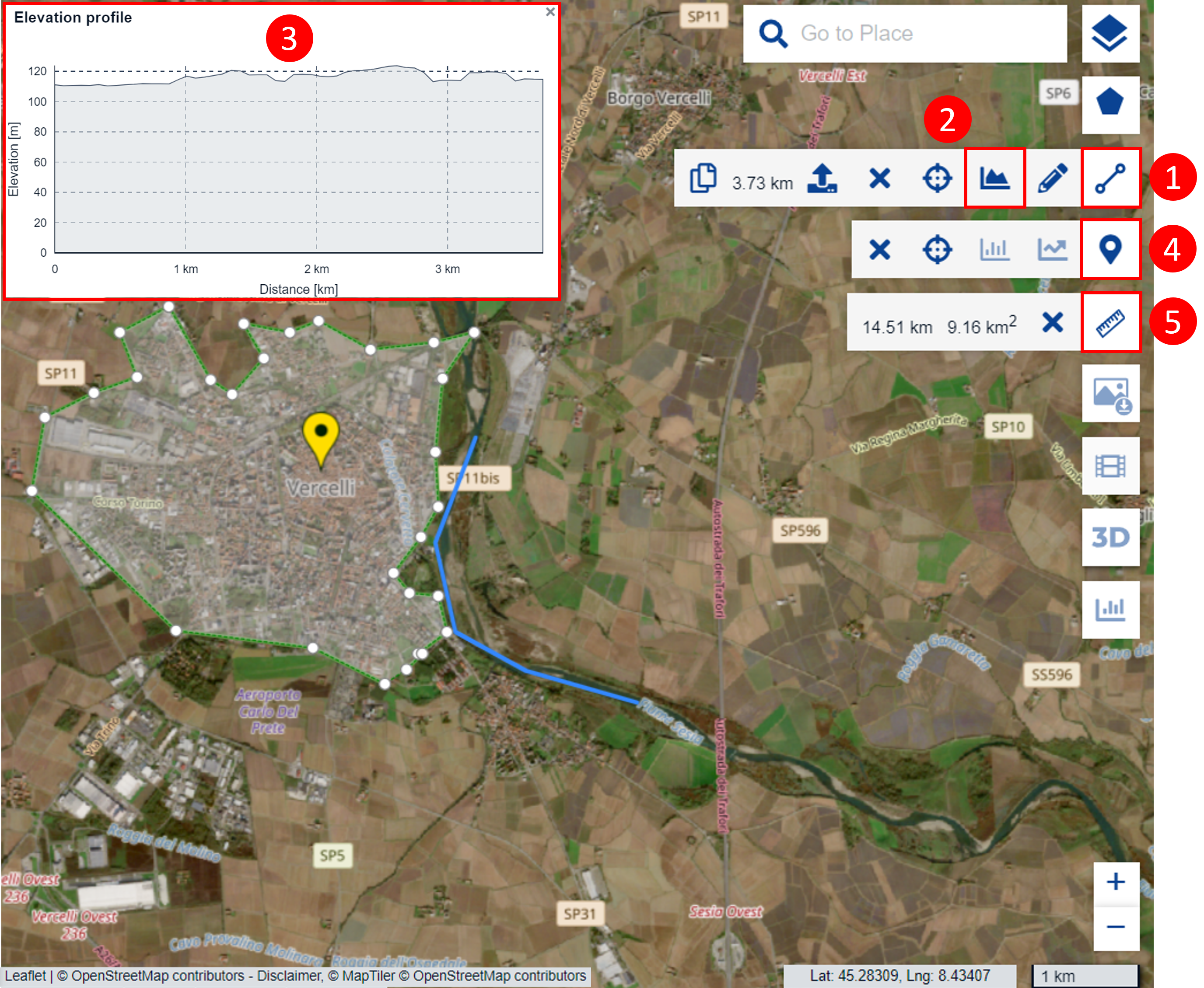
Fig. 2.1.2.5 – Draw a line, Mark point of interest and Measure tools
2.1.2.1. Registration in Copernicus Browser
From here click on Login (1) (Fig. 2.1.2.6), as you can see another window will pop up with the option to Log-in (if you already have an account) or register. In order to create an account click on Register (2). Now fill the mandatory fields as shown, keep in mind that your password must contain at least 1 special character, 1 upper case character, 1 lower case character, 1 numerical digit and have a minimum length of 12. Once you have finished click on Register (3). At this point you will receive an email (on the email you have set in the registration form) requiring you to verify your address. In order to do so follow the indicated steps. If you have not received any email try to look into your Spam or Junk folder.

Fig. 2.1.2.6 – Registration in Copernicus Browser
2.1.2.2. Logged in Copernicus Browser and language change
Once you are logged in (Fig. 2.1.2.7), your name will appear on the top right corner of the sidebar (1); on its left side of it (2) you can set your preferred language.

Fig. 2.1.2.7 – Logged in Copernicus Browser and language change
2.1.2.3. How to select correct products with Copernicus Browser
Now we will configure the searching parameters (Fig. 2.1.2.8):
- Search for the Area of interest (1), our study area is “Piedmont, Vercelli, Italy”
- Click on SEARCH (2)
- We are looking for Sentinel-2 images. Therefore, Check Sentinel-2 (3) as a data source
- Now check L2A (4), limiting the search only toward Sentinel-2 atmospherically corrected images
- Set the Maximum cloud coverage (5) to 35%
- Set the TIME RANGE
- regarding the date component (dd-mm-yyyy) set both From and Until to “03-10-2020” (6)
- for the hour and minutes component set it From 00 hh and 00 mm Until to 11 hh and 00 mm (7)
- Click the Search (8) button
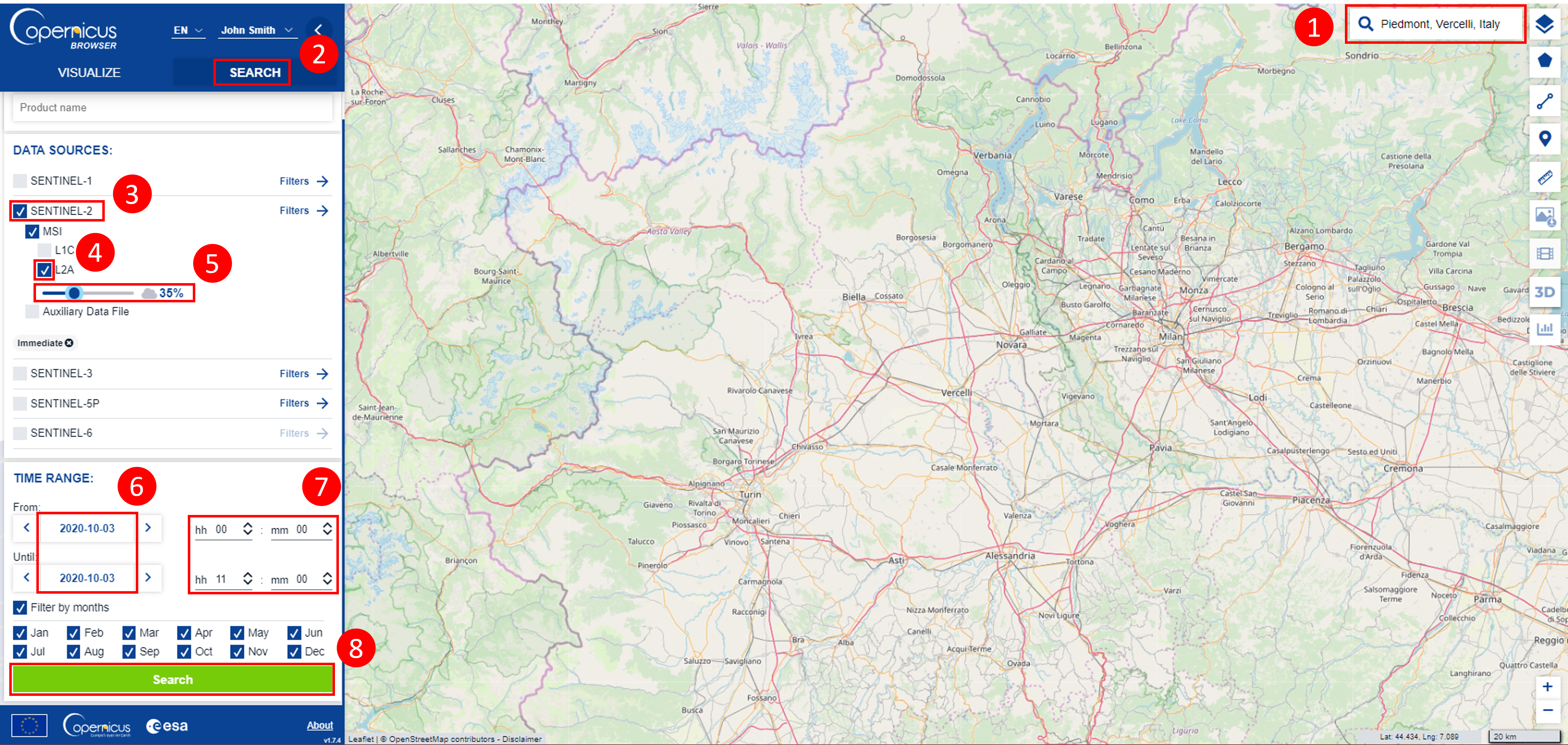
Fig. 2.1.2.8 – Select the correct products in Copernicus Browser
2.1.2.4. How to view the satellite images with Copernicus Browser
Select the desired image footprint
The area on the Earth that was visible to the satellite at the time of taking the image is displayed as a polygon. Here you can inspect the full metadata of the image tiles by clicking on the product info button (1) Now, you can visualize your chosen product either by selecting the desired image tile (2) (image taken over Vercelli) in the main window or by clicking Visualize (3) on the sidebar. (Fig. 2.1.2.9) Details of the image that we are looking for are reported here:
- Product type: Sentinel-2 L2A
- Date: 03-10-2020
- Time: 10:17:59 UTC (Hour: min: sec)
- Cloud cover percentage: 33.8%
- Tile ID: 32TMR
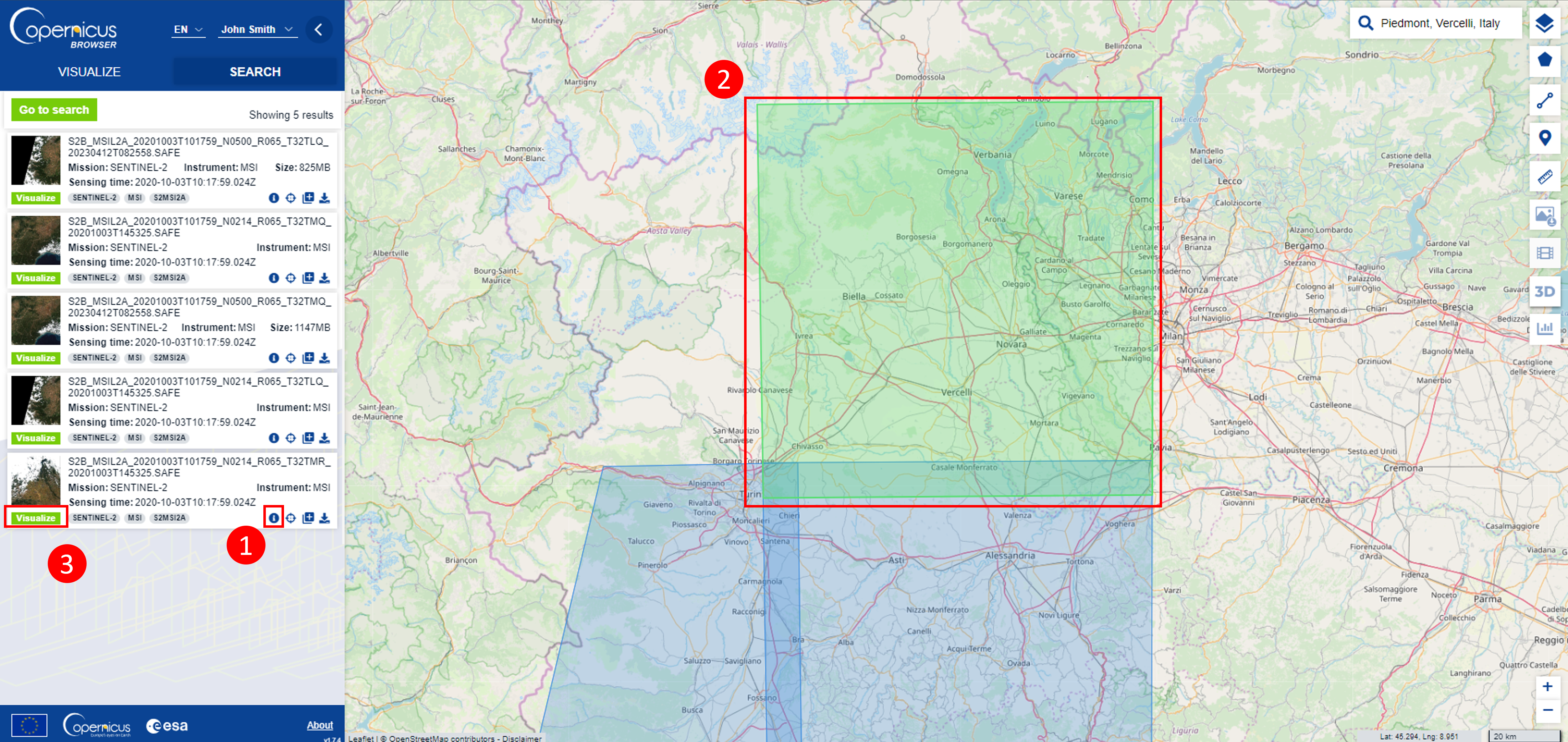
Fig. 2.1.2.9 – Selection of the desired Satellite image from Copernicus Browser map panel
The product summary is visible in Fig. 2.1.2.10.
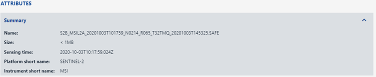
Fig. 2.1.2.10 – Desired image details